Cost Issues of Near Real-Time Offline Data Warehouses - Incremental Data Warehouse Series Part I
Demand for Near Real-Time Offline Data Warehouses
The offline data warehouse, especially the Spark + Hive computing and storage architecture, has undergone more than ten years of development and industry validation, becoming the de facto standard in the industry. However, with the industry’s increasing demand for data timeliness, a real-time computing and storage architecture based on Flink + various types of storage has gradually developed. Due to different usage scenarios, costs, and data processing accuracy, this has led to the widespread use of the Lambda architecture in the industry to this day. (Interestingly, Hive, Spark, and Flink respectively won the SIGMOD system awards in 2018, 2022, and 2023.)
Whether from intuition or the pursuit of mathematical beauty, it seems that everyone believes that architectures like the Kappa architecture should be able to achieve harmonious unification of both approaches. Unfortunately, there are very few cases of successful implementation in the industry. There are many reasons for this, and in this article, we will analyze the cost issues from the perspective of near real-time offline data warehouses.
The additional cost issues brought by making offline data warehouses near real-time seem to be a simple and intuitive conclusion: if you want better timeliness, you need to pay some additional costs. This article will attempt to organize answers to the related cost issues based on existing papers.
Formalizing Additional Costs of Near Real-Time Offline Data Warehouses Through Incrementality
Through model comparison, this article selects the SIGMOD'20 paper Thrifty Query Execution via Incrementability (“Thrifty Query Execution via Incrementability”) as the model explanation. One reason for this selection is that the model in this paper is simpler and easier to understand (which is why we didn’t choose more complex papers like Tempura for explanation).
Problem Description: How to minimize overall computational processing costs while meeting data timeliness requirements.
This is the core concept of this article. Real-time processing timeliness can achieve end-to-end second-level performance, while offline data warehouse processing timeliness is T+1. Clearly, offline data warehouse timeliness is too poor, but in most scenarios, we don’t actually need second-level timeliness—most people who obtain information from data warehouses for decision-making cannot respond at second-level speeds. Therefore, on one hand, we need to improve timeliness, but on the other hand, we only need to meet actual requirements. We will provide the mathematical expression for this problem later.
The following are the terminology definitions needed to explain this problem:
Final work: Data processing completion for querying, which can be seen as data timeliness. In the offline context, this corresponds to data ready time. Note that due to often lengthy offline data warehouse chains, the ready time for final ADS layer data is not the ideal T+1, but often the morning or even noon of the next day.
Total work: All costs paid to make data queryable, which can be seen as job running core*hour.
To achieve better timeliness (reduce final work), we often need to pay additional costs (additional work)
This needs to be explained with the following diagram: for example, if our final work is 10 AM the next day, and we hope to advance the data timeliness to before 7 AM the next day, to achieve this effect, we need to perform advance calculations. Since the results of advance calculations are not completely consistent with the final results, some of this work becomes additional costs—in other words, it increases additional work. The reason why advance calculation results are not completely consistent with final results can be illustrated with the max aggregation function—its intermediate max value does not necessarily represent the final max value with day as the dimension. In other words, there are some intermediate “useless” processing operations. In Flink’s general stream computing framework, we call these “finally useless” intermediate output results the changelog model, where those intermediate results that are ultimately useless will send update-before information to downstream systems, reminding them to delete previous results, which is called retracting previously sent messages.

Query path: Data exchange nodes, data reading, and data output nodes for executing query processing. Corresponds to a chained operator node in Flink or a stage in Spark. In the simplest algorithm, different operators can decide how much data to accumulate before sending to downstream systems. By adjusting configurations of each operator, dynamic optimization can be achieved. In Flink’s real-time scenarios, by default no data is accumulated, per-record sending achieves the highest timeliness but also the highest additional computational costs; in mini-batch scenarios, we can avoid some useless advance processing by calculating within each batch.
Pace: On each query path, pace=1 means execution only once (corresponding to offline scenarios where calculation occurs only once at the end in batches), pace=k means sending downstream only after collecting 1/k of the data (the larger k is, the more frequent incremental calculation becomes, usually resulting in higher additional costs).
Incrementability: Incrementality. We can reduce final work (improve data visibility) through advance incremental calculation. However, this must be considered based on costs, so we use benefit of extra total work to measure Incrementability:
This simplifies the entire processing model, measuring Incrementability only through the single variable pace. $P_{2}$ produces different Incrementability effects compared to $P_{1}$ on this query path.
Incrementability = ∞ Complete incrementality: Operations without retraction issues, such as filter, map, etc., where previous incremental calculations are not wasted. To improve timeliness, no additional costs are needed.
0 < Incrementability < ∞ Partial incrementality: Retraction operations exist, where previous incremental calculations may no longer be needed, so additional costs are required to improve timeliness. This includes a large number of aggregation operations and join operations.
Mathematical formulation of our problem (how to minimize overall computational processing costs while meeting data timeliness requirements):
The entire cost model aims to minimize total work under the constraint of timeliness coefficient $L$. Using near real-time data warehouse description, this means minimizing costs under certain timeliness conditions. For example, if our coefficient is 0.7, meaning if data is ready at 10 AM, we need to advance it to at least 7 AM, how to adjust pace on different query paths to optimize costs as much as possible. The $Cost_{final_work}(1)$ on the right side of the formula represents the offline data warehouse scenario where all operations are calculated only once (pace = 1) in batch processing.
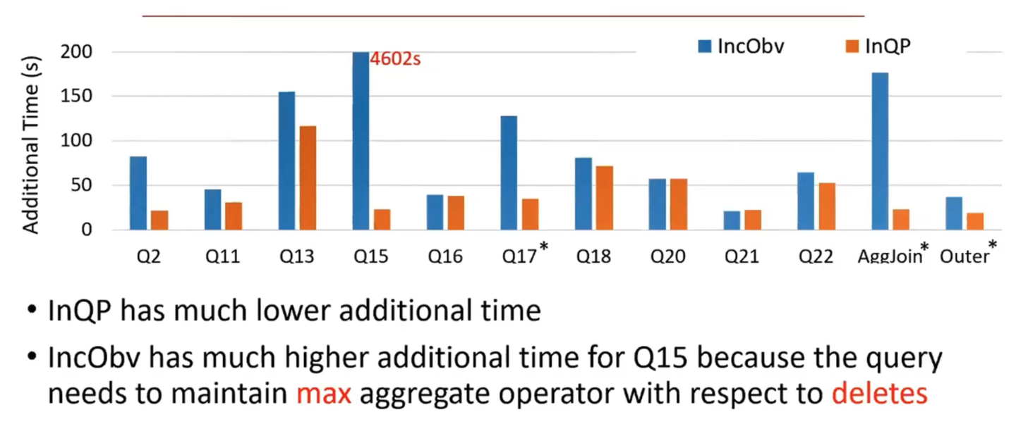
The optimization method in the paper configures different pace values for different query paths through algorithms to obtain an optimal solution. The blue line on the left side of the figure below is the baseline obtained by fixing all query paths to the same pace value (corresponding to Spark’s fixed micro-batch size), while the orange line is the optimized algorithm. For example, TPC-H Q15 involves max calculation retraction, resulting in significant additional work costs.
We can also use this theory to explain why the cost of partial update processing methods is low. If data lake partial update is used, then Flink’s additional work (we only discuss left join operations, not considering retractions from other field processing) becomes 0, while the data lake performs batch processing of left join behavior during compaction intervals, equivalent to minimizing pace as much as possible, making overall costs controllable.
Theory Guiding Practice
After analyzing this model, let’s return to the current scenario of near real-time offline data warehouses:
| Daily Incremental Table Situation | Input Data Volume | Total Work | Additional Work Analysis in Total Work | Final Work | Pace |
|---|---|---|---|---|---|
| Offline Processing | Size(day_inc) | Trigger only when data is ready: $Cost(batch_T)$ | 0, no retraction issues | Late data ready time: $Cost(batch_F)$ | 1 |
| General Real-time Processing Represented by Flink | Same as offline = Size(di) | Additional work due to aggregation processing: $Cost$ > $Cost(batch_T)$ | For aggregations, retractions exist; for DWD layer widening left joins, retractions exist; write amplification from compaction for better read performance in intermediate states is also a cost. Cost(t’) > 0 | Data ready time can be advanced < $Cost(batch_F)$ | Source → Aggregation operators and Source → Join operators pace approaches ∞, meaning eager processing per record; Aggregation operators → Downstream operators pace is k, determined by mini-batch size |
| Full Data Table Situation | Input Data Volume | Total Work | Additional Work Analysis in Total Work | Final Work |
|---|---|---|---|---|
| Offline Processing | Size(full) | Trigger when data is ready: $Cost(batch_T)$ | 0, no retraction issues | Late data ready time, some important tables need to wait until 3 AM $Cost(F)$ |
| General Real-time Processing Represented by Flink | Incremental data Size(day_inc) < Size(full) | Since processed data volume is less than full table, cost may be less than $Cost$ <? $Cost(batch_T)$ | For aggregations, retractions exist. For DWD layer widening left joins, retractions exist. Write amplification from compaction for better read performance in intermediate states is also a cost. $Cost(t’)$ > 0 | Data ready time can be advanced significantly < $Cost(F)$ without considering cross-cloud transfer costs |
It can be seen that for full data tables (tables that have existed since system inception), implementing incremental data warehouses through real-time processing theoretically has cost advantages. However, another issue is obvious: general real-time frameworks represented by Flink, in real-time processing, require storing permanent states for stateful operators due to full data processing. This is unacceptable for Flink’s computing processing model (currently LSM compaction is extremely unfriendly to infinite TTL). Even with the yet-to-be-developed disaggregated state storage in Flink-2.0, the cost remains unacceptable.
So, what good solutions do we have? Please look forward to subsequent articles in the incremental data warehouse series.